

A healthcare operations team with 480 labeled adverse-event records can produce a credible demo in six weeks by fine-tuning a pretrained model. The same model fails in production when it meets a rare drug interaction, a missing lab value, or a clinician note outside the training pattern. This pattern repeats across low-data machine learning. Teams start with a pretrained model, get a strong demo metric, then learn that the business case depends on the edge cases where the model has the least evidence.
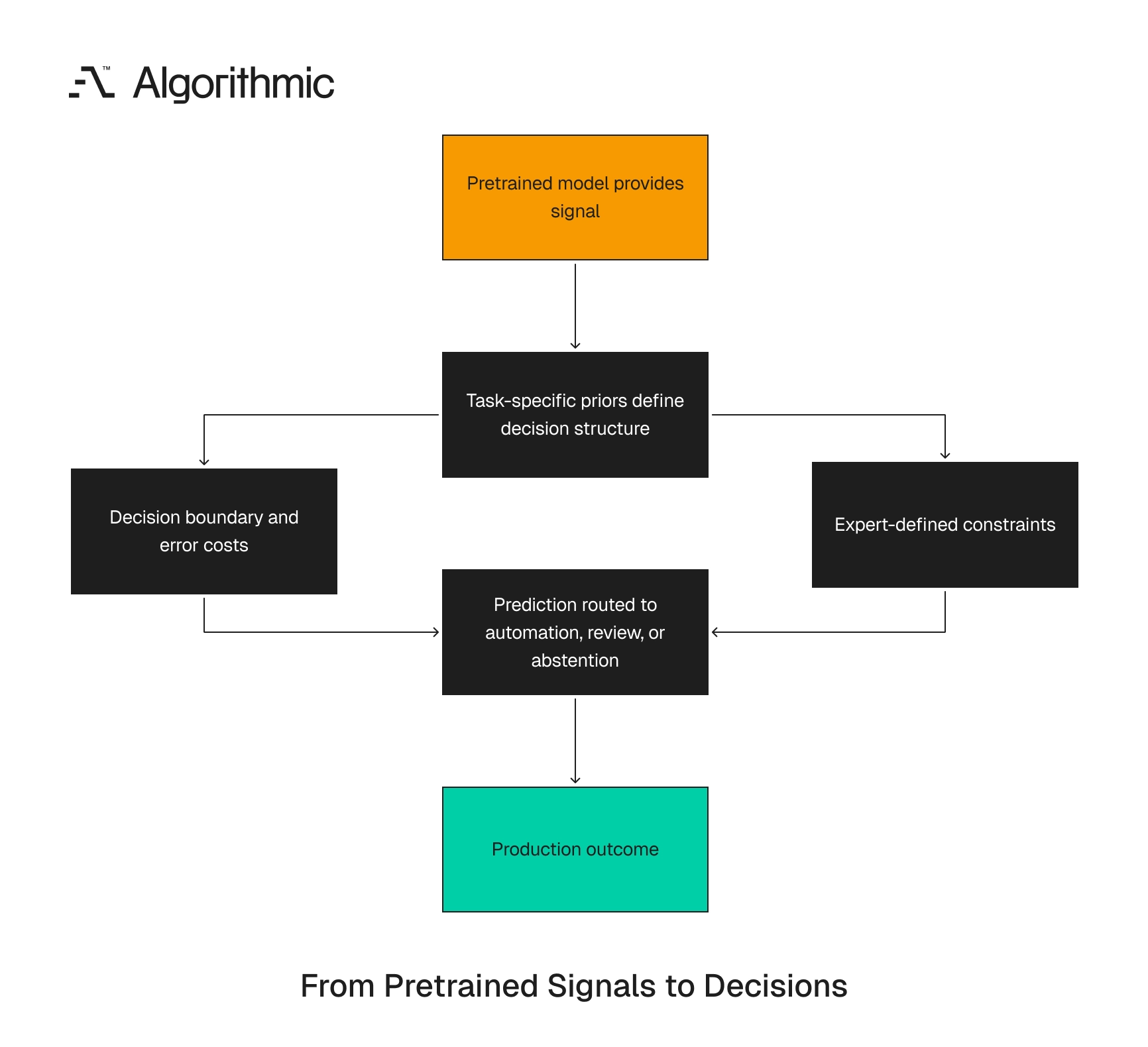
Algorithmic’s operating rule is priors before pretraining. A prior is a formal assumption that constrains learning, stating which outcomes are plausible, which errors are expensive, which measurements deserve trust, and where expert review is mandatory. Pretrained models supply signal, and priors form the control plane that turns that signal into a defensible decision. This rule applies across predictive analytics work in industrial, healthcare, scientific, and specialized enterprise workflows, where labels are expensive, error costs are high, and historical records rarely describe the decision with enough precision.
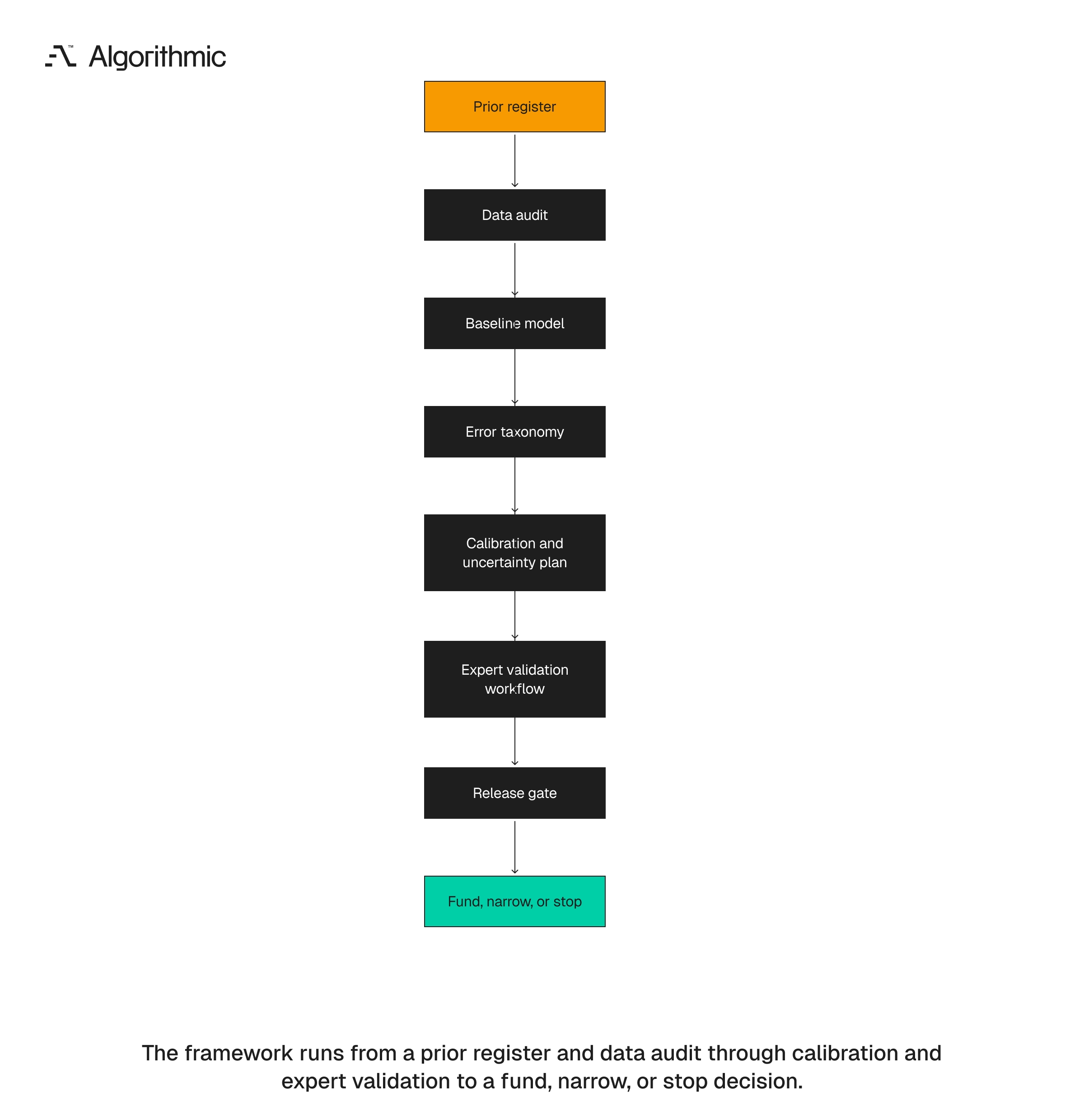
Historical data also reflects inconsistent process, changing equipment, and expert judgment that was never recorded. In these settings, model choice matters only after the team defines the task with enough detail to test it. A six-month build without that work creates avoidable risk, while a 30-day feasibility phase with a prior register, data audit, baseline model, and release gate gives leaders a funding decision before sunk cost accumulates. Low-data machine learning fails when teams treat pretraining as a substitute for decision design.
Pretrained models supply representations and priors supply task structure
Pretrained models encode statistical patterns from large corpora. In computer vision, that means ImageNet features learned from millions of labeled images. In language, it means token relationships learned across web-scale text. In tabular prediction, it means embeddings learned from historical enterprise records. These representations help when the target task resembles the training distribution, and they give less protection when the business case depends on narrow domain rules, rare events, or asymmetric error costs.
A model trained on broad patterns lacks the business context to rank operational risk. It can recognize a phrase, image feature, or sequence pattern without knowing the decision rule. A recent paper on transfer learning with informative priors shows why this matters, since transfer performance improves when prior information is explicit instead of buried inside a model checkpoint. A pretrained model can recognize that a maintenance note mentions “bearing vibration”, while a domain prior states when that phrase changes the operational decision, and that distinction determines whether the system creates a useful work order or noise.
Vibration above a threshold matters only when load, temperature, and operating hours fall within defined ranges, and it also depends on sensor age, calibration history, and maintenance state. The first function supports a demo, while the second supports a work order, shutdown decision, or human review queue. A production system needs both, since the pretrained model extracts a useful representation and the prior defines the decision boundary that representation must respect.
 Click to expand
 In one industrial setting, a vibration phrase meant little during a planned spin-down sequence, and the same phrase triggered review during stable load above 70% of rated capacity. That distinction was a prior, expressed as a rule and tested against historical work orders, and the model had no reliable way to infer it from 14 failure records. This is the central low-data constraint, since sparse labels rarely contain enough evidence to teach the model the operating policy, so the team must state the policy directly.
The same pattern appears in healthcare, where a note that mentions “shortness of breath” means different things after surgery, during chemotherapy, and during a routine primary-care visit. A language model can identify the phrase, and the clinical prior defines which patient state, medication history, and lab pattern make that phrase clinically relevant. Scientific workflows show the same issue, since a model can detect an anomalous peak in assay data while the prior defines whether the peak violates known chemistry. In low-data systems, representations compress evidence and priors define acceptable action.
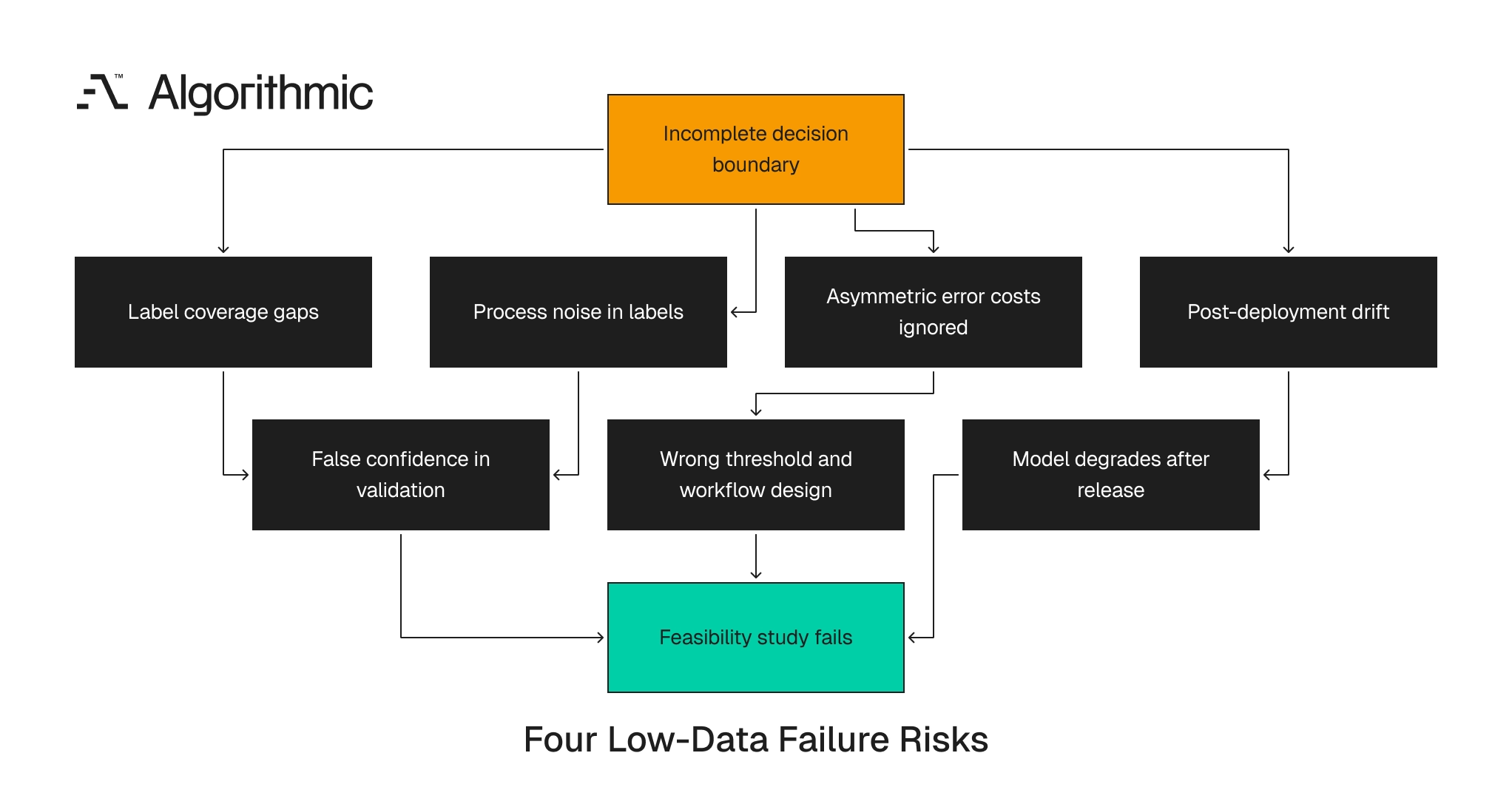
Low-data settings fail through four mechanisms
Low-data projects fail in repeatable ways, and the failure rarely starts with PyTorch, TensorFlow, or model architecture. It starts with an incomplete task description, where the model receives labels without a precise account of the decision, the cost of error, or the limits of measurement. The four mechanisms below account for many production failures in scarce-data settings, and each requires a different engineering response. Treating all four as “more data” problems wastes labeling budget and delays the moment when leadership learns whether the use case deserves funding. A disciplined feasibility phase separates these failure modes early and gives the team a repair plan before a model becomes the center of the program.
 Click to expand
 The label set does not represent the decision boundary
A team can have 2,000 labeled examples and still have inadequate coverage. If 85% of labels come from normal operating conditions, the model learns normal process variation and has limited evidence for shutdown conditions, equipment transitions, rare faults, and abnormal human interventions. Validation performance then reflects the easy portion of the process.
This matters in industrial inspection. A defect classifier trained on 1,500 images from one production line can perform well on a random validation split, then fail on the second line when lighting, camera angle, and operator behavior change the image distribution. The validation split did not test the production shift. The validation score reports performance on available labels, while the business needs performance on the cases that trigger cost, safety exposure, warranty claims, or regulatory review.
A useful data audit separates label volume from decision coverage. Teams count examples by fault type, site, operator, equipment state, time period, and product family, because if a safety-critical class has 12 examples, an accuracy number across all classes has limited value, and that class deserves targeted review before fine-tuning starts. The audit also needs negative evidence, so teams should identify operating conditions where a failure cannot occur, where a sensor cannot report, or where a label has no meaning. A component cannot fail after 4,000 hours if it was replaced at 3,500 hours, and if the dataset says otherwise the record needs repair before training.
Random splits hide this issue, while time-based splits, site-based splits, and equipment-based holdouts expose whether the model generalizes to the decision environment. The audit should produce a coverage matrix rather than a single label count, with rows for decision conditions and columns for sites, time periods, and product groups. A practical matrix often changes the project plan, since a team with 50,000 records can discover that only 37 records cover the high-cost failure mode. That discovery prevents a common error, because the team stops treating the total dataset as evidence for a decision that appears in one narrow slice.
The labels encode process noise
Many enterprise labels are downstream artifacts. A customer churn label can reflect sales coverage as much as customer intent, a clinical escalation label can reflect bed availability and physician preference, and a quality failure label can reflect which technician inspected the unit. Training directly on these labels teaches the model the historical process, and the model then repeats prior inconsistency with mathematical confidence.
The fix starts with a noise model that distinguishes measurement error, human disagreement, missing data, and delayed outcomes. Measurement error requires sensor review, recalibration, or field exclusion, and human disagreement requires adjudication and clearer label definitions. Missing data requires workflow analysis and feature availability checks, while delayed outcomes require time-aware labeling because late labels create leakage.
A churn model shows the issue, since if cancellation notes appear after the customer has left, the model learns a future event, performs well offline, and fails at the point of decision. The offline score measures access to leaked information instead of predictive value. A clinical model carries the same risk, because if a discharge-risk label reflects a case manager’s later note, the model learns documentation behavior, and the production workflow needs a prediction before the note exists, so the feature set must match that moment exactly.
A low-data team cannot absorb label noise through scale. With 500 labels, 50 noisy records can move thresholds, distort calibration, and change executive conclusions. Noise also changes which model class looks best, since a high-capacity model often fits inconsistent labels faster than a constrained baseline, which creates a false ranking during evaluation because the model appears stronger only because it learned the defects embedded in the process. The team should audit labels as work products, giving each label a source system, creation timestamp, reviewer identity where available, and known delay. A label without provenance deserves lower trust, and in high-cost workflows those labels should be excluded, adjudicated, or separated during evaluation.
The cost of error is asymmetric
Most business ML problems treat false positives and false negatives differently. A false fraud alert creates customer friction and a missed fraud event creates financial loss, a false medical risk alert consumes clinician time, and a missed high-risk patient can create patient harm and regulatory exposure. Accuracy collapses these tradeoffs into one number, while precision, recall, calibration, expected cost, and abstention rate give decision makers a better operating view.
A production machine learning team defines the loss function with the business owner before model training begins, and the metric must reflect the workflow where the model will run. For a safety workflow, recall for high-cost events can outweigh average accuracy, and for an analyst queue, false positives can dominate because staff capacity is fixed. Expected cost makes the tradeoff explicit, so if a false negative safety event costs 20 times a false positive, the threshold must reflect that ratio. That threshold needs approval from the business owner, and it belongs in the architecture decision record, model card, and release gate.
The team should also translate the threshold into operational load, because a model that flags 9% of cases can overwhelm a review team staffed for 3%. This is a production design issue, since the model, queue, staffing plan, and escalation policy form one decision system. A low-data model with a calibrated abstention path often beats a model that forces a score for every record, because high-cost workflows need permission to say “expert review required”.
A useful release plan converts error rates into operating numbers, so leaders see expected false alerts, missed events, reviews per week, and escalation load. A threshold with 92% recall can still create 1,200 weekly reviews, and if the expert team can handle 300, the design fails operationally. This arithmetic belongs in the feasibility study, since it prevents a model team from celebrating a metric that the business cannot use.
The data changes after deployment
Low-data models face drift early because the original sample was narrow. New equipment, product categories, clinicians, markets, and customer behavior change the input distribution, so a model trained on one quarter of sensor data can fail after a planned maintenance cycle, and a clinical model trained before a protocol change can misread later patient pathways. This is why ML systems in production need monitoring and drift detection from the first release, because a low-data system without drift detection loses trust every week.
Monitoring covers input distributions, missingness, prediction scores, subgroup metrics, and outcome feedback, and the team sets alert thresholds before launch. The first release also includes a retraining policy that defines who approves new training data, when labels mature, and how prior assumptions are retested. Without this operating model, the team has a static model inside a changing process, and low-data systems need active measurement from day one.
Drift monitoring must connect to an action path, because an alert without an owner becomes noise after the third week. A practical policy names the reviewer, the trigger threshold, the incident record, and the rollback decision, and it defines when retraining is allowed. In regulated or high-cost workflows, retraining without approval can create more risk than drift, so version control, holdout testing, and sign-off are part of the operating model.
Drift also affects priors, since a prior written for one product generation can fail after a component redesign or supplier change. The monitoring plan should test both data drift and prior violation rates, and if rule violations rise, the system needs review before the model is retrained. Retraining a model on a changed process does not repair a stale operating assumption.
The low-data prior framework
A low-data ML feasibility study should produce a prior register before any fine-tuning run. The register records the assumptions that constrain the model, the evidence behind them, and the test that verifies them. This artifact changes the project conversation, moving the team from model selection to decision defensibility, which improves technical planning and executive review and gives the buyer a concrete basis for funding or stopping the build.
| Prior category | Concrete question | Example | Production test |
|---|---|---|---|
| Domain constraint | Which outcomes are impossible or rare under known conditions? | A component cannot fail before 50 operating hours unless installation was incomplete | Rule violation rate under batch scoring |
| Measurement trust | Which fields, sensors, or labels have known error rates? | Temperature sensors drift after 18 months without recalibration | Sensor-age stratified error analysis |
| Error cost | Which mistakes require human review or abstention? | False negative safety events cost 20x false positives | Expected cost per 1,000 predictions |
| Population structure | Which subgroups need separate evaluation? | New sites, elderly patients, low-volume SKUs | Subgroup calibration and recall |
| Temporal behavior | Which signals must precede the outcome? | Maintenance note after failure cannot train failure prediction | Leakage audit by timestamp |
| Expert override | Where does human judgment supersede the model? | Clinician review for high-uncertainty discharge recommendations | Override rate and reason codes |
The register should be short enough for executive review and precise enough for engineering work, and in most feasibility studies six to ten priors expose the main risks. Each prior needs an owner, so a process engineer owns equipment constraints and a clinical lead owns medical review rules. A data lead owns timestamp and feature availability assumptions, and the ML lead owns how those assumptions enter training, evaluation, calibration, and release gates.
The 2025 Journal of Big Data survey on machine learning with small and limited data covers the methods available for scarce-data settings, and the operating lesson is narrower, since method selection follows a written account of priors, label noise, and evaluation risk. A prior register also improves vendor control, because it gives the buyer a concrete artifact to review before a large model build receives funding.
The register should use testable language, since “sensor quality varies” is too vague for engineering work. “Temperature sensors older than 18 months drift by more than 2 degrees Celsius unless recalibrated” can be tested, and it can become a feature rule, monitoring check, or exclusion criterion. The register also prevents silent scope expansion, because if a use case lacks enough evidence for full automation, the team can fund a review queue instead, which often produces value faster and creates labeled outcomes that support a later automation decision.
A strong prior register is specific, owned, and linked to a test. Specific language prevents interpretation drift across engineering, domain, and executive teams, ownership prevents assumptions from becoming anonymous project notes, and testing turns the register into an engineering control. A prior that cannot be tested belongs in a research note, not a release gate.
 Click to expand
 The register should also record how each prior enters the system, since some priors become hard rules while others affect sampling, calibration, abstention, or monitoring. This matters because priors are not all equal, so a physical impossibility deserves a hard exclusion while a clinician preference deserves review and measurement.
Model selection after priors are explicit
Pretrained models remain useful in low-data work, and they enter the architecture after the team has defined the structure of the problem. This order reduces wasted experimentation and prevents teams from accepting a strong demo metric that fails the operational decision. The selection sequence is direct, so the team builds an interpretable baseline, tests leakage, adds representation learning where it helps, and constrains the decision layer with priors. Model selection should answer whether added complexity improves the decision enough to justify its operating cost, which includes infrastructure, monitoring, audit support, release review, and incident response, and in low-data settings those costs often exceed initial training cost.
Start with interpretable baselines
A logistic regression model, gradient boosted trees, or a monotonic model can expose data leakage, unstable features, and label noise quickly. In tabular risk scoring, tree-based models such as XGBoost often provide a strong first benchmark within two weeks. Baselines also give experts something to inspect, since a domain expert can review feature importance, partial dependence, and error clusters, and this review often finds data defects that a larger model would absorb silently, such as a top feature that is a timestamped status field recorded after the event.
A transparent baseline sets a cost floor, because if a small model performs within five points of a fine-tuned model, the larger system needs a clear production reason. For a 90-day feasibility study, the first milestone should be a baseline model, an error taxonomy, and a prior register, and fine-tuning should follow that milestone. The baseline should include subgroup evaluation, since overall accuracy can hide poor recall for new sites, rare SKUs, elderly patients, or late-shift production runs.
A baseline exposes the economics of complexity, so a three-feature model that captures 70% of value can justify a narrow release, while a fine-tuned model with higher offline performance carries more operational cost through monitoring, calibration, version control, inference infrastructure, and audit support. The comparison belongs in the funding decision, framed as the incremental value of added complexity measured against the decision and workflow.
Baselines also force the team to define evaluation clearly, since a random split, time split, site holdout, and subgroup report can produce different conclusions. A mature team shows all four when the decision requires them, which reduces surprise when the first release meets real production variation. The baseline should be reproducible, so the team records code version, data snapshot, feature list, split method, and metric definitions, which prevents a common failure during fine-tuning where teams cannot explain whether improvement came from the model, the split, the features, or a changed dataset.
Use pretraining for representation, then constrain decisions
A pretrained vision model can extract useful image features from 300 inspection images, and a pretrained language model can embed 5,000 support notes. These representations can feed smaller supervised models, retrieval systems, or expert review queues, while the decision layer still needs domain constraints. A model predicting equipment failure should respect maintenance windows, operating hours, and known failure modes, and it should know which sensor readings are unavailable during downtime. A model predicting clinical deterioration should report uncertainty and abstain when required fields are missing, never forcing a risk score when the evidence is incomplete.
Research on non-generative prior extraction from language models points to a related direction, since pretrained models can contain useful prior information that can be extracted without turning the system into an unconstrained generator. For enterprise use, the extraction process needs audit logs and validation against domain experts, because a generated prior without expert approval creates a new source of hidden error.
The practical architecture is direct, using the pretrained model for feature extraction and explicit priors for the workflow decision. The decision layer can be a calibrated classifier, a rules engine, a Bayesian model, or a queueing policy, and the right choice depends on the action attached to the prediction. In our review of low-data systems, this separation reduces avoidable debate, since the team stops arguing about model size and starts testing where decisions can be trusted.
This architecture also improves auditability, because a reviewer can inspect the representation source, decision rule, uncertainty score, and override reason separately. Separation helps incident response too, since if a model misses a failure, the team can test whether the representation failed or the decision rule was incomplete. That diagnostic structure matters for regulated workflows, because a single opaque score gives the team fewer repair paths after an incident.
Use semi-supervised and unsupervised pipelines
Low-data projects often have few labels and many unlabeled records, a pattern common in manufacturing images, sensor histories, case notes, customer transcripts, and scientific measurements. Semi-supervised learning can use unlabeled data to learn structure before supervised training, clustering can reveal subpopulations, anomaly detection can identify rare patterns for expert review, and self-supervised learning can build representations from unlabeled images or time series. Contrastive learning can separate normal and abnormal operating patterns before labels exist, and these methods change which labels are worth buying.
A manufacturing team with 100,000 unlabeled images and 600 labels should avoid random labeling and use clustering and anomaly scores to sample rare conditions. A customer operations team with millions of support notes can cluster complaints before training a churn model, so experts label cluster-level patterns instead of isolated tickets. This approach reduces wasted labeling and gives the team a better view of subgroup coverage before supervised training begins.
The sampling plan should be explicit, and a practical plan can allocate 40% of new labels to rare clusters, 30% to model-confident errors, and 30% to production-volume cases. This balance protects the team from overfitting to anomalies and keeps evaluation tied to the cases that dominate production load. Unlabeled data also exposes process drift before launch, since if recent records form a separate cluster, the historical labels no longer represent the current workflow.
The team should preserve cluster assignments and anomaly scores as audit fields, which help reviewers understand why a case entered the labeling queue. These fields also support later monitoring, because a rise in one cluster can indicate a new product issue, documentation change, or sensor problem. Semi-supervised work still needs a decision frame, since better representations do not replace priors, calibration, or expert review.
Treat active learning as a guided probe
Active learning selects examples for labeling based on model uncertainty or expected information gain, and it works best when the team already has a clear error taxonomy and stable expert review. It fails when asked to discover the full structure of an unknown domain, because the model can query only where its current representation sees uncertainty, so rare failure modes outside that representation can remain invisible, which is dangerous in safety, fraud, clinical, and industrial inspection work.
Use active learning to test specific hypotheses, such as whether the model confuses early corrosion with lighting artifacts on Line 3. That question produces better labeling work than a broad request to label uncertain cases, and it gives experts a defined review standard. Active learning should have a stop condition, so if new labels no longer reduce a target error category, the team redirects labeling budget to another failure mode.
The label queue needs capacity planning, since an active learning system that sends 800 cases per week to three experts will degrade label quality. A feasible process defines daily review volume, review time per case, adjudication rules, and escalation paths, because without these constraints active learning becomes unplanned manual labor. The queue should also include control cases, where a small percentage of known examples tests reviewer drift and label consistency over time, so a clinical review queue can insert 20 previously adjudicated cases each month and use changes in reviewer decisions to reveal training gaps or definition drift. Active learning is an operating process, not a model setting, so it needs staffing, quality checks, budget rules, and a defined endpoint.
Expert validation is part of the model architecture
Expert-in-the-loop design is often treated as an annotation task, but in low-data ML it is part of the architecture. Experts define priors, review disagreements, set abstention rules, and approve failure taxonomies, and their input should be captured as structured data instead of scattered comments in a project channel. This requires a workflow instead of a weekly meeting, one that records reviewer identity, decision reason, confidence, evidence source, and final adjudication. The architecture should treat expert review as a production component with queue design, service-level targets, audit fields, and feedback loops into training data, and it should make the boundary between automation and supervision visible in metrics, release notes, and user training.
Build a disagreement protocol
A reliable validation process records where experts agree, where they disagree, and why. A medical workflow can require two clinicians and an adjudicator, and an industrial workflow can require a technician, a quality engineer, and a process owner, where each reviewer sees the same evidence package and label definition. Inter-rater agreement should be measured, so Cohen’s kappa or Krippendorff’s alpha can show whether the label definition is stable enough for supervised learning. If experts disagree on 30% of reviewed cases, model performance has a ceiling imposed by the label process, and more training runs will not remove that ceiling.
The disagreement protocol should separate ambiguity from error, since an ambiguous case needs an abstention path while a mislabeled case needs correction and audit history. This distinction matters during model evaluation, because penalizing the model for cases that experts cannot label consistently gives a false picture of technical performance, so the evaluation set should tag ambiguous cases separately. The protocol should also define who can change a label after release, and in regulated workflows post-hoc label edits need reviewer identity, reason code, and timestamp, which protects both the team and the business owner and lets the organization learn from incidents without rewriting history.
The protocol should include a review cadence, since weekly adjudication works for feasibility while production workflows often need daily review for high-risk queues. It also needs escalation criteria, so a disagreement involving safety exposure moves to a named owner within a defined time window. These details determine whether the model learns from expert judgment or from inconsistent project communication.
Calibrate uncertainty before release
A low-data model must know when to abstain, and calibration measures whether predicted probabilities match observed outcomes. A model that assigns 80% risk should be correct about 80% of the time within that risk band, which matters when users route work by confidence level. Calibration can be assessed with reliability diagrams, Brier score, and expected calibration error, and these measures matter because production workflows often route predictions by confidence. A model with 92% accuracy and poor calibration can create unsafe automation, while a model with 84% accuracy and reliable abstention can be safer in a supervised workflow.
Calibration should be measured by subgroup, since a risk score calibrated for all patients can still be miscalibrated for elderly patients or a new clinic. The release gate should specify acceptable calibration error, abstention rate, and subgroup recall, tied to workflow capacity and error cost. The calibration plan also needs a minimum sample rule, because a subgroup with 18 examples cannot support a confident release decision, so the release path should narrow the workflow, require expert review, or collect more data until production confidence matches the evidence base.
Calibration should be tested after threshold selection, since a model can look calibrated across the full score range and still fail near the operating threshold. That threshold region matters most, because it determines which cases enter automation, review, or no-action paths. Teams should inspect uncertainty bands with domain experts, who often find that high-uncertainty cases align with missing fields, rare states, or ambiguous labels.
Keep an audit trail
Every prediction in a regulated or high-cost workflow should include model version, input data version, feature set, uncertainty score, and decision outcome, which is standard MLOps engineering. Auditability also helps teams improve, because when a model fails the team needs to identify the failure source, which can be drift, label noise, missing priors, data leakage, or an invalid assumption, and each cause has a different repair path. A drift failure requires monitoring and retraining review, a label noise failure requires process correction, a missing prior requires a change to the decision architecture, and a leakage failure requires feature removal and historical re-evaluation.
The audit trail should be queryable by incident, subgroup, model version, and time period, since screenshots and manual notes are inadequate for regulated or high-cost workflows. Audit fields should be designed before launch, because retrofitting them after an incident creates incomplete records and weakens root-cause analysis. For practical teams, this means storing prediction records in a durable table instead of a logging side channel, so the table becomes the operating memory of the ML system.
The audit schema should include user action, since a prediction that users routinely override has a different risk profile from one they follow. Override data can become training evidence after adjudication, and it can reveal poor workflow design, unclear alerts, or distrust caused by earlier errors. A useful audit trail answers three questions, namely what the model knew, what the human did, and what happened later.
A 30-day feasibility plan for low-data ML
A technical founder or enterprise leader should avoid approving a six-month build without a 30-day feasibility phase, whose goal is to decide whether the available data supports the intended decision. This phase ends with a funding decision, and the answer is continue, stop, or repair the data process before model development proceeds. The plan below is the minimum operating sequence we expect for low-data predictive systems, short enough for executive review and specific enough for engineering work. It assumes a small senior team of one ML engineer, one data engineer, one domain lead, and one business owner, and for regulated workflows it adds a compliance reviewer during Week 1, since waiting until release review creates rework and weakens the evidence record.
Week 1 covers prior and workflow definition
Document the decision being made, the user who acts on the prediction, and the cost of each error type, then build the prior register with domain experts. Identify fields or labels with known quality problems, recording any field that is manually entered, delayed, overwritten, or produced after the decision point. The output should include an architecture decision record, a metric plan, and a list of assumptions that require testing, and it should name the owner for each assumption. The team should also define the intervention tied to the prediction, because a prediction without a specific action creates evaluation ambiguity and weak production adoption.
This week sets the release posture, so the team decides whether the first version recommends, triages, alerts, or automates, since those are different systems with different risk profiles and a triage queue can tolerate more uncertainty than a fully automated action. Week 1 should also define the unit of prediction, which in healthcare can be a patient encounter, a 24-hour period, or a discharge event, and in manufacturing can be a part, batch, machine-hour, or inspection image, because misstating this unit causes label leakage and metric confusion. The team should write one sentence that links prediction to action, for example that at 06:00 daily the model ranks discharge-risk cases for nurse manager review, since that sentence anchors the rest of the feasibility study by defining timing, user, action, and review path.
Week 2 covers data audit and leakage test
Profile missingness, duplicates, label delay, timestamp consistency, and subgroup coverage, then check whether outcome information appears in features unavailable at prediction time. Many predictive analytics projects fail here, since a model predicting churn can learn from cancellation notes created after the customer already left, and a model predicting equipment failure can learn from maintenance actions recorded after the failure, so both models look effective offline and fail during live use. The audit should produce a feature availability matrix that marks each feature as available before, during, or after the decision point, and it should quantify subgroup coverage, because if one site contributes 70% of the data, evaluation must separate that site from the others.
The audit should end with a red, yellow, or green rating for each feature group, where red features are excluded, yellow features need review, and green features can enter baselines, which gives leaders a fast read on data readiness and prevents late arguments about why a high-performing feature was removed. Week 2 should include a label provenance review that identifies who created labels, when they were created, and which system stored them, and it should test duplicate logic, since duplicate patients, parts, customer accounts, or service tickets can inflate validation scores. A practical leakage test retrains the baseline after removing suspicious features, and if performance collapses, the team has found a decision-time mismatch, a useful result that directs funding toward data repair instead of model complexity.
Week 3 covers baseline model and error taxonomy
Train a transparent baseline, then review false positives, false negatives, and high-uncertainty cases with experts. Create a taxonomy with five to ten error categories that are operational instead of statistical abstractions, such as missing calibration records, ambiguous clinician notes, rare equipment state, duplicated customer accounts, and delayed outcome labels, and give each category an owner and proposed remedy. The taxonomy should drive the next data decision, because if 40% of errors come from missing sensor calibration records, more labels will not fix the issue, the data pipeline needs repair, and labeling more examples from the same defective process only makes the model learn the defect more confidently.
The baseline review should identify the lowest-risk release path, since a model that performs well for one site and poorly for four sites can support a site-limited pilot written as a constrained release rather than a general production deployment, because scope discipline protects the organization from overclaiming early results. Week 3 should include a calibration check even for a preliminary model, since early calibration work exposes whether scores can support triage, and the team should compute expected operating load, because a threshold that flags 600 weekly cases has different staffing needs from one that flags 80. Experts should review representative errors rather than only the most extreme ones, which prevents the team from designing around anecdotes, and by the end of Week 3 leaders should see the main failure modes and which ones are data, policy, or model problems.
Week 4 covers pretraining tests and release gate
Run a constrained pretrained-model experiment after the baseline, comparing performance by subgroup, uncertainty band, and expected cost. Test whether unlabeled data improves representation quality, using clustering, anomaly detection, or self-supervised representations where unlabeled volume supports the work. The release gate should be explicit, including minimum recall for high-cost cases, maximum abstention rate, calibration target, drift monitoring plan, and expert review path, and it should state stop conditions, so if subgroup recall falls below the safety threshold, the project moves to data repair or workflow redesign.
A 30-day study should not produce a full production system, only evidence that the production system deserves funding, so the final readout should be an investment memo rather than a model demo, stating the decision, evidence, risks, cost, release scope, and next funding gate. If the answer is stop, the study has succeeded, since it prevented a longer build from turning weak data into expensive software. Week 4 should also define the first production boundary, which can limit sites, users, product lines, patient groups, or decision types, and the team should state what the model will not handle in the first release, with exclusions appearing in user training, monitoring, and support documentation. The readout should include a clear funding path, since leaders need to know the cost of production build, data repair, expert review, and monitoring, and a credible plan separates those costs because bundling them into one model estimate hides the operating burden of low-data systems.
Vendor evaluation for scarce-data ML
Low-data ML exposes the difference between senior ML systems teams and fine-tuning vendors, and the distinction appears in the first technical conversation. Use this checklist when evaluating a machine learning development company or MLOps engineering team.
- They can state the domain priors before naming a model family.
- They ask for label provenance, inter-rater agreement, and timestamp semantics.
- They propose baselines before large-model fine-tuning.
- They discuss semi-supervised learning, anomaly detection, or self-supervised representations where unlabeled data is abundant.
- They define uncertainty quantification, calibration, and abstention rules.
- They include expert validation inside the system design.
- They require audit logs, model versioning, and drift monitoring.
- They can explain when active learning will help and where it will fail.
- They produce a feasibility plan with gates, metrics, and stop conditions.
- They refuse to promise production reliability from a demo dataset.
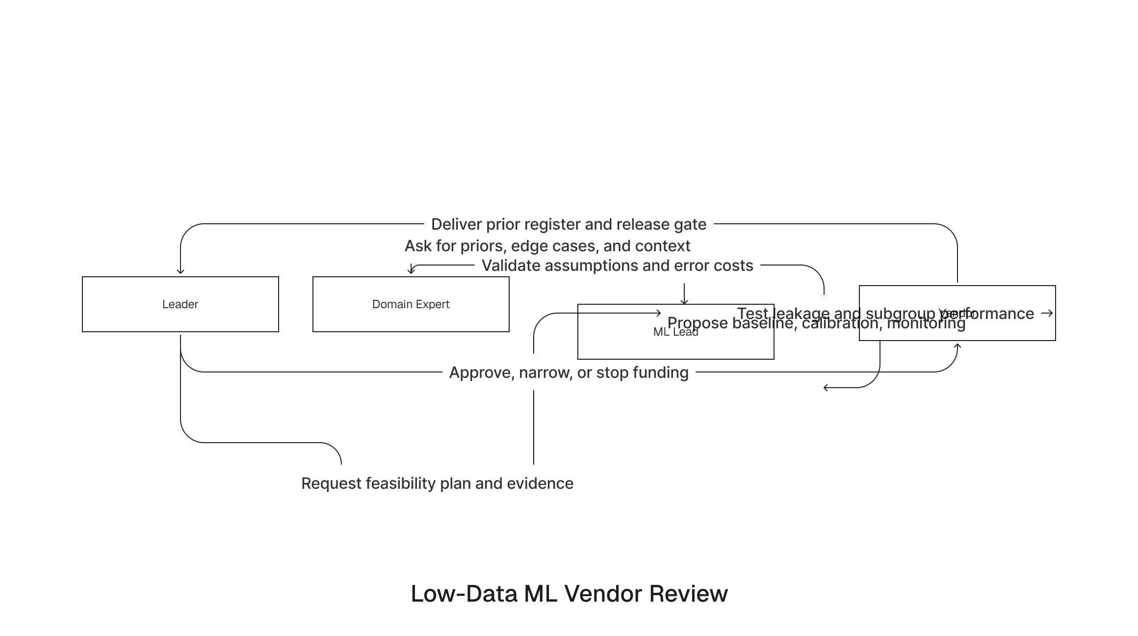
A vendor that starts with a pretrained model and ends with a validation accuracy number has skipped the work that determines production reliability. A senior software development team makes uncertainty visible early, because hidden uncertainty becomes operational risk. The strongest teams challenge the requested use case, so if the data cannot support the decision, they recommend a narrower workflow, an expert review queue, or data collection first. This is risk control, since a failed six-month build costs more than a 30-day stop decision. The buyer should ask for artifacts instead of assurances, and the required artifacts are a prior register, data audit, baseline model, error taxonomy, calibration plan, and release gate.
 Click to expand
 The buyer should also ask how the vendor handles disagreement, since a vague answer about expert review signals weak operating design. A credible answer names the reviewers, adjudication rule, data fields, quality metrics, and audit trail, and it explains how disagreements change the training set and release gate. The contract should reflect these artifacts, because payment milestones tied only to model delivery create pressure to preserve a weak use case, while milestones tied to evidence quality create better incentives and give executives a clean way to stop, narrow, or expand the build.
Procurement should test how the vendor handles unfavorable findings, since a senior team will state that a use case lacks evidence when the data says so. Ask for an example of a stopped project, because the answer reveals whether the vendor protects the client’s capital or only sells delivery hours. The statement of work should include decision gates, where a gate after the data audit gives the buyer an exit before fine-tuning starts, a second gate after baseline review prevents the team from scaling a weak model, and a third gate before production release verifies calibration, monitoring, and review readiness. These gates reduce commercial ambiguity and align the vendor with the evidence needed for production trust.
What leaders should do next
Low-data ML remains a task of assumption design, measurement discipline, and expert validation, and rising adoption of predictive analytics does not reduce that engineering burden. The same discipline that separates strong ML work from thin work also shapes feature engineering, which decides machine learning outcomes long before model choice. Before approving fine-tuning work, require a prior register, a label-noise assessment, an uncertainty plan, and a 30-day feasibility study, and fund the model build only after those artifacts show that the decision can be made safely with the available data.
Leaders should assign ownership before the first model run, so the business owner owns error cost, the domain expert owns priors, the data lead owns feature availability and label quality, and the ML lead owns model design, calibration, monitoring, and release gates. This division prevents a pretrained model from becoming a substitute for decision design. The immediate directive is direct, since a leader should not approve a low-data ML build from a demo metric, and should instead ask for the prior register, data audit, baseline error taxonomy, calibration plan, and release gate. If the team cannot produce those artifacts in 30 days, the organization is not ready for a production model.
Low-data machine learning succeeds when the team makes assumptions explicit, tests them early, and treats uncertainty as an engineering object, which turns scarce data into a controlled production decision. The right next step is operational, not theoretical, so select one candidate use case and run the 30-day feasibility sequence before funding production work, then use the result to set the release boundary. Continue only when the evidence supports the decision, the workflow can absorb the output, and the owners accept the error profile.
Algorithmic runs predictive analytics feasibility work that builds the prior register, data audit, and release gate before any fine-tuning run. Start a conversation if you are weighing a low-data model and want to know whether the data supports the decision before you fund the build.