Hyperparameter optimization to maximize ML performance

In enterprise machine learning, achieving baseline model accuracy remains a primary bottleneck. In addition, the structural challenge is optimizing the model to deliver maximum business yield without incurring prohibitive compute costs (OpEx). Most ML projects follow a standard trajectory, where data is engineered, a model is trained, and the initial results are acceptable - but they are almost always suboptimal. At this juncture, technical leadership faces a capital allocation decision (between time and resources). They can either deploy the baseline model (accepting margin leakage via sub-optimal predictions) or invest engineering cycles into Hyperparameter Optimization (HPO).

Hyperparameters are the architectural constraints that dictate how a model learns. Tuning them is a strategic lever to increase predictive accuracy by 2 to 10%. However, because HPO consumes major GPU compute and engineering bandwidth, brute-force tuning is a structural error. This expanded blueprint provides a strategic framework for evaluating hyperparameter tuning as an economic trade-off, detailing search methodologies, multi-objective optimization, and infrastructure governance.

Diagnosing the problem of parameters versus hyperparameters

A pervasive point of friction between business stakeholders and data science teams is a fundamental misunderstanding of what engineering can directly control during model development.

• Model parameters (Output): These are the internal variables (weights, biases, coefficients) that the algorithm learns autonomously from the data. Engineers do not (and must not) set these manually.
• Hyperparameters (Constraints): These are the structural settings configured before training initiates. They govern learning velocity, architectural complexity, and regularization aggressiveness.

If a machine learning model is an engine, the data is the fuel, the parameters are the internal combustion dynamics the engine develops through operation, and the hyperparameters are the electronic control unit (ECU) settings that govern those dynamics. Engineers configure the ECU before the engine runs. The engine’s internal behavior emerges from the interaction between that configuration and the fuel it processes. Setting the correct hyperparameter values dictates whether a model extracts generalizable market patterns or simply memorizes historical noise (overfitting).

The ROI baseline and why tuning is a strategic imperative

Hyperparameter optimization sits at a specific, high-impact point on the effort-to-impact curve. While feature engineering remains the primary driver of baseline performance, tuning acts as the yield multiplier.

According to foundational research published in the Journal of Machine Learning Research (JMLR), proper tuning yields an additional 2-5% performance lift for tree-based architectures and upwards of 10-15% for complex neural networks.

At enterprise scale, these percentages translate directly to the bottom line:

• Manufacturing (Risk Mitigation): A 2% reduction in the false-negative rate of a visual inspection model prevents millions in product recalls.
• FinTech (Revenue Protection): A 3% precision improvement in a transaction fraud detection model directly reduces capital write-offs without increasing customer friction.
• E-Commerce (Unit Economics): A 5% lift in a recommendation engine’s click-through rate directly scales average order value (AOV) and revenue-per-session.

As established by industry leaders like Andrew Ng, the optimal capital allocation for modeling effort is typically 70-80% focused on data quality and feature engineering, with a strict 20-30% time-boxed reserve for hyperparameter optimization and validation.

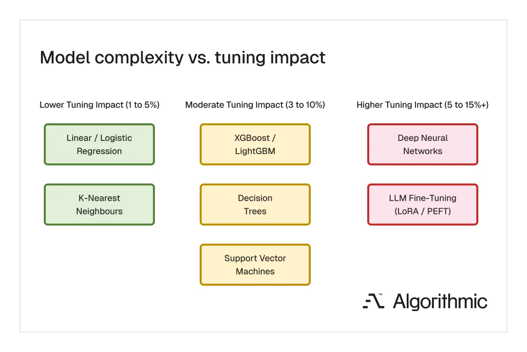
The impact of hyperparameter tuning varies notably across model classes. Simpler architectures with fewer configurable settings tend to yield modest gains. Complex architectures with large search spaces offer the greatest potential improvement and justify the greatest tuning investment.

Click to expand

Architectural levers and key hyperparameters by model class

The required compute investment for tuning scales non-linearly with model complexity. Technical leaders must understand which levers carry the highest operational impact, spanning from legacy statistical models to modern Large Language Models (LLMs).

Linear and logistic regression (low compute cost)

Standard linear models are highly efficient but prone to overfitting if unconstrained.

• Regularization Strength (L1/L2 Penalties): Controls the strictness of the model. Strong penalties reduce overfitting but may miss subtle data patterns; weak penalties capture detail but risk memorizing noise.
• Solver Selection: According to scikit-learn documentation, selecting the right algorithmic engine is critical. saga is structurally required for massive datasets, whereas lbfgs is optimal for smaller, dense matrices.

Tree-based ensembles - XGBoost & LightGBM (medium compute cost)

Gradient boosting machines build a sequence of decision trees. They remain the enterprise standard for structured tabular data.

• Learning Rate (Shrinkage): Scales the impact of each sequential tree. Lower rates yield highly reliable models but require exponentially more computing time.
• Maximum Depth: Controls architectural complexity. Shallow trees (depth 3-6) generalize reliably while deep trees memorize training data.
• Subsampling (Rows & Columns): Injecting mathematical randomness by restricting the data each tree can access, fundamentally reducing model variance.

K-nearest neighbors (low-to-medium compute cost)

KNN makes predictions by comparing a new data point to its closest neighbors in the feature space. It remains effective for smaller structured datasets and delivers interpretable results, though inference cost scales linearly with data volume.

• Number of Neighbors (K): The single highest-impact lever. A low K value makes the model reactive to local noise, producing unstable predictions. A high K value smooths the decision boundary and stabilizes output, at the cost of losing sensitivity to localized patterns.

• Distance Metric: Defines how the algorithm calculates similarity between data points. Euclidean distance performs well on continuous, normalized features. Manhattan distance is structurally better suited for high-dimensional or sparse feature spaces where outlier sensitivity must be controlled.

• Weighting Scheme: Determines whether all neighbors contribute equally to the prediction or whether proximity grants disproportionate influence. Distance-weighted predictions consistently improve accuracy on datasets with imbalanced class distributions.

Support vector machines (medium compute cost)

SVMs construct a decision boundary (hyperplane) that maximizes the margin of separation between classes. They perform reliably on medium-sized, structured datasets and can model non-linear relationships through kernel transformations.

• Kernel Selection: The kernel function transforms input data into a higher-dimensional space where linear separation becomes feasible. A linear kernel is sufficient for linearly separable problems. The Radial Basis Function (RBF) kernel captures non-linear boundaries. Polynomial kernels offer configurable complexity but increase overfitting risk at higher degrees.

• Regularization (C): Governs the trade-off between margin width and classification accuracy on training data. A high C value forces the model to classify training examples correctly, narrowing the margin. A low C value permits some misclassification in exchange for a wider margin and stronger generalization to unseen data.

• Gamma: Controls the radius of influence of a single training example. Low gamma values produce broad, smooth decision boundaries suited to generalization. High gamma values produce tightly contoured boundaries that conform closely to individual data points, increasing the risk of overfitting. As documented in scikit-learn’s SVM guide, the interaction between C and gamma is the primary tuning priority for RBF kernels.

Deep neural networks & LLM fine-tuning (high compute cost)

Neural networks model highly non-linear relationships in unstructured data (vision, language) but require massive GPU OpEx to tune. In the modern era of Generative AI, Parameter-Efficient Fine-Tuning (PEFT) introduces net-new hyperparameters.

• Batch Size & Learning Rate Schedulers: The volume of data processed before weights update, combined with dynamic step sizes (e.g., Cosine Annealing), dictates convergence speed and stability.
• LoRA Rank (r) and Alpha: When fine-tuning foundation models using Low-Rank Adaptation (LoRA), the r parameter determines the dimensionality of the update matrices, establishing a direct trade-off between model adaptability and VRAM consumption.

Each search methodology occupies a different position on the compute cost versus search precision spectrum. The choice depends on model complexity, available infrastructure, and the number of hyperparameters under optimization.

Click to expand

Strategic countermeasures such as search methodologies

With potentially an infinite number of hyperparameter combinations, brute-force search is an indefensible misallocation of compute capital. Organizations must mandate efficient search methodologies.

• Grid search (Brute force approach): Exhaustively tests every defined combination. Only acceptable for simple models with fewer than three variables. For complex systems, the computational cost grows exponentially.
• Random search (Stochastic efficiency): Seminal research by Bergstra and Bengio (2012) proved that Random Search achieves equal or superior accuracy to Grid Search using a fraction of the compute cycles. This should be the default baseline for standard ML teams.
• Bayesian optimization (Directed ROI): Builds a probabilistic surrogate model to predict which hyperparameter combinations will yield the highest return, actively learning from past failures. Mandatory for deep learning, where a single training run takes hours.
• Coarse-to-fine search (Staged precision): A hybrid method that sequences random and grid search across multiple stages. The process follows a disciplined cycle of defining broad hyperparameter ranges, executing a random search across the full space, identifying the regions where strong performance concentrates, and then executing a tighter grid or random search within those narrowed regions. This cycle repeats until convergence. The method captures the exploration efficiency of random search during the early stage and the thoroughness of grid search where it matters most. It is particularly effective for neural networks and gradient boosting ensembles with large, continuous search spaces, where a single-pass search method would either be too expensive (grid search) or too imprecise (random search).
• Population-based training (PBT): Pioneered by DeepMind, PBT trains a population of models concurrently, dynamically transferring successful hyperparameters from high-performing models to underperforming ones during the training run, drastically reducing wall-clock time.

Multi-objective optimization for tuning beyond accuracy as a metric

A frequent oversight in data science is tuning exclusively for predictive accuracy (e.g., F1-score or RMSE). In enterprise production environments, accuracy is only one dimension of business value. HPO must be structured as a Multi-Objective Optimization problem.

Leaders must force teams to define the Pareto Frontier, the mathematical curve that represents the optimal trade-off between competing metrics.

When tuning, teams must simultaneously optimize for:

1. Predictive accuracy: The core business logic.
2. Inference latency: A model with 99% accuracy is useless in high-frequency trading or real-time bidding if inference takes 500 milliseconds. Hyperparameters such as tree depth and the number of network layers directly affect this latency.
3. Memory footprint: For edge deployment (IoT, mobile applications), hyperparameter tuning must constrain the final size of the model weights to fit within strict hardware limitations.
4. Algorithmic fairness: Tuning parameters so error rates do not disproportionately impact protected demographic cohorts, a regulatory requirement under the EU AI Act.

AutoML versus custom pipeline dilemma

As the MLOps tooling ecosystem matures, technical leadership faces a classic “Build vs. Buy” decision regarding hyperparameter tuning: Automated Machine Learning (AutoML) versus custom, orchestrated search pipelines.

• The AutoML advantage: Platforms like Google Cloud Vertex AI, DataRobot, and AWS SageMaker Autopilot abstract HPO entirely. They automatically select algorithms and tune hyperparameters via proprietary backend infrastructure. This is strategically viable for teams with high data volume but constrained engineering talent, accelerating time-to-market.
• The custom pipeline mandate: AutoML operates as a “black box”, making it unsuitable for highly regulated industries (banking, healthcare) where precise auditability of the tuning process is legally mandated. Furthermore, at massive scale, the licensing costs of proprietary AutoML platforms often exceed the OpEx of running custom, open-source tuning frameworks (like Optuna or Ray Tune) on raw compute.

Open-source tuning frameworks: a comparative overview

For organizations that mandate custom pipelines, three open-source frameworks dominate the current tooling space.

Ray Tune is a Python library designed for distributed hyperparameter tuning at scale. It integrates natively with PyTorch, TensorFlow, XGBoost, and scikit-learn, and supports search algorithms from Optuna, HyperBand, and Bayesian backends. Its primary structural advantage is parallelization: Ray Tune distributes trials across multiple CPUs, GPUs, or cluster nodes, reducing wall-clock time in direct proportion to available hardware. It is the strongest option for teams operating multi-node infrastructure and running large-scale search campaigns.

Optuna implements Bayesian optimization through a lightweight, define-by-run API. It supports automated pruning (early termination of unpromizing trials), parallelized search, and provides a real-time web dashboard for monitoring optimization history and hyperparameter importance rankings. Its low infrastructure overhead makes it a practical default for teams that want directed search without deploying a full distributed compute framework.

Weights & Biases (W&B) sweeps integrates hyperparameter tuning directly into the experiment tracking workflow. It supports grid, random, and Bayesian search methods, logs all trial results automatically, and provides visualization tools for analyzing hyperparameter interactions and identifying diminishing-return thresholds. The integration with W&B’s broader experiment tracking platform reduces the metadata management burden that typically accompanies large tuning campaigns.

The selection between these frameworks depends on infrastructure maturity, team size, and the scale of the search. Ray Tune suits teams with distributed compute resources running hundreds or thousands of trials. Optuna suits teams that need efficient directed search on a single machine or small cluster. W&B Sweeps suits teams that prioritize experiment traceability and collaborative visibility across the modeling lifecycle.

Operationalizing the search - cost-reduction and ESG frameworks

Hyperparameter tuning should never be a blank check. Before initiating a tuning pipeline, engineering leads must enforce optimization protocols to protect cloud margins and follow corporate ESG (Environmental, Social, and Governance) mandates.

• Representative subsampling: Running tuning trials on a stratified 20% sample of the training data reduces per-trial compute costs by 80%. Once optimal bounds are identified, final validation is performed on the full dataset.
• Domain-informed range constraints: Understanding typical effective ranges for specific model types eliminates a large volume of wasted trials before the search begins. For XGBoost and LightGBM, learning rates rarely need to exceed 0.3 or fall below 0.001 for structured tabular data. In production practice, neural network batch sizes range from 16 to 512 for datasets that fit within GPU memory. Regularization strength for logistic regression typically ranges from 0.001 to 100. LoRA rank values for LLM fine-tuning range between 4 and 64 commonly, with diminishing returns above 32 for most downstream tasks. Starting with these empirically validated ranges rather than arbitrary bounds reduces the effective search space by an order of magnitude, as outlined in Google’s Machine Learning Engineering best practices guide.
• Early stopping mandates: For iterative models, infrastructure must be configured to automatically terminate training runs that plateau early. Paying for GPU time on a mathematically doomed configuration is value leakage.
• Configuration transfer from prior projects: If the organization has tuned similar models on related datasets, those historical configurations provide high-quality starting points that compress the search timeline. This is particularly valuable for teams that maintain ML experiment tracking infrastructure (MLflow, Weights & Biases, Neptune). Over time, accumulated hyperparameter configurations become institutional knowledge: a searchable record of which settings worked for which model-data combinations, eliminating redundant exploration across projects. The compounding value of this institutional memory increases with each successive project, making experiment tracking infrastructure an investment that pays dividends well beyond individual model deployments.
• Green AI and carbon tracking: As documented by the Allen Institute for AI in their foundational paper Green AI, the carbon footprint of extensive hyperparameter tuning is staggering. Organizations must integrate carbon tracking metrics into their MLOps pipelines, forcing data scientists to justify the environmental cost of running thousands of GPU-intensive trials for a marginal 0.1% accuracy gain.

ML model and managing hyperparameter drift

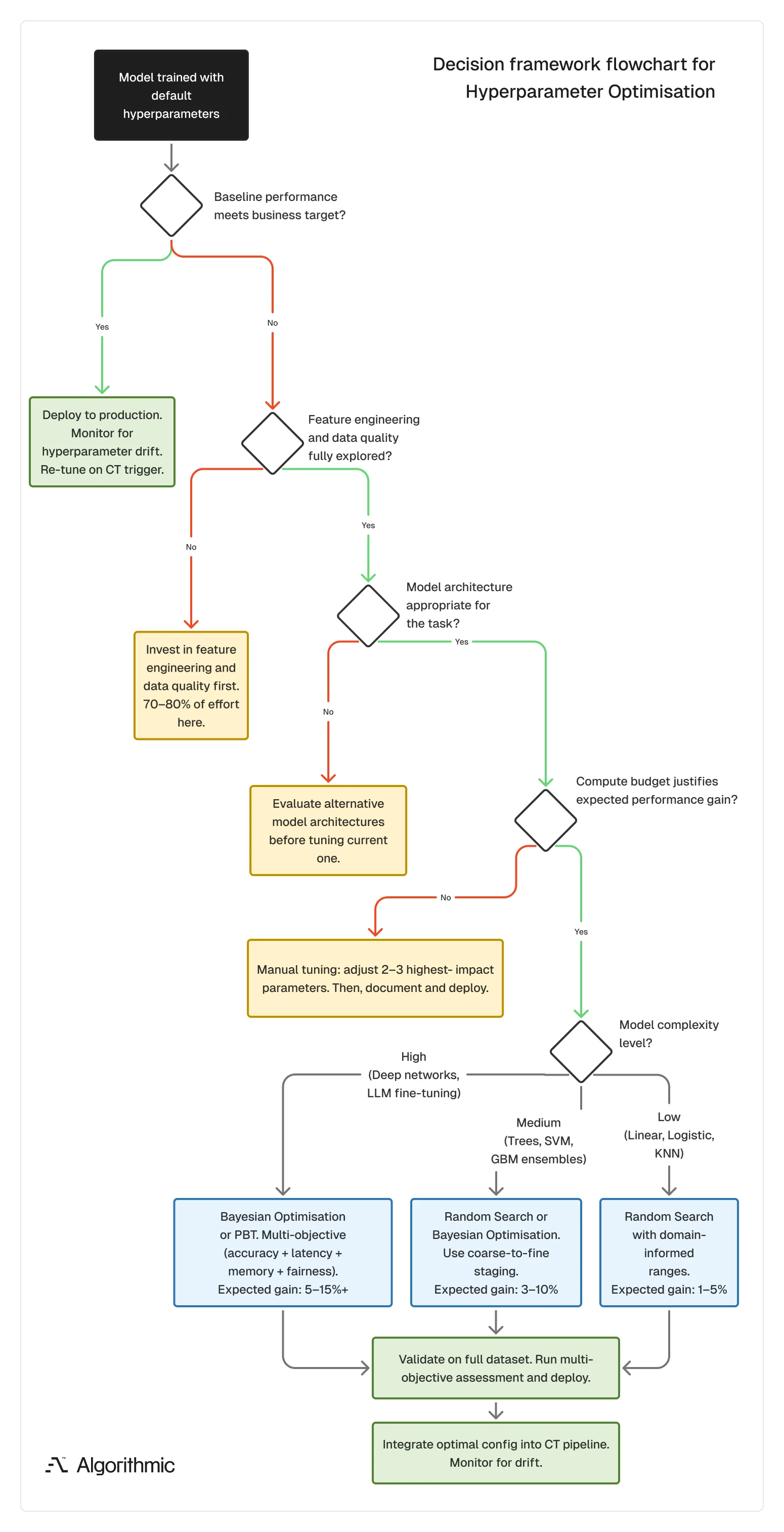
A critical fallacy in enterprise AI is assuming that hyperparameter optimization is a one-time event executed prior to deployment. In reality, as external market conditions evolve, the underlying data distributions change (Data Drift). A model trained with a learning rate and regularization penalty optimized for Q1 data will likely be structurally misaligned with Q4 data. To maintain operational resilience, hyperparameter optimization must be integrated into the Continuous Training (CT) pipeline. When drift is detected, the automated pipeline should retrain the model weights on new data and re-trigger a bounded hyperparameter search so the model architecture adapts to the new market reality.

The following decision flow helps technical leadership determine whether hyperparameter optimization is the right next investment or whether engineering cycles are better allocated upstream to data quality and feature engineering.

Click to expand

The tuning decision matrix

Before committing infrastructure to hyperparameter optimization, organizations must evaluate a rigid economic equation.

Does the projected business value of the performance gain exceed the sum of the compute OpEx, the engineering opportunity cost, and the environmental impact?

Some checkpoint questions that can be helpful:

1. Define your performance target: What metric improvement would change a business decision? If a 2% accuracy gain does not materially affect the downstream application, extensive tuning is misallocated effort. If that 2% prevents a system failure or recovers major revenue, it warrants a disciplined search.
2. Assess model and data complexity: Complex architectures (deep networks, large ensembles) with high-dimensional data and large search spaces benefit most from structured tuning. Simpler models on well-understood data often perform adequately with default or manually selected values.
3. Audit available resources: Tuning techniques, even parallelized ones, require CPUs, GPUs, and engineering time. Estimate total compute hours before starting. If the projected cost exceeds the projected value of the performance gain, defer tuning in favor of feature engineering, data quality improvements, or model selection experiments.

When the expected gain matches the required investment, hyperparameter tuning becomes a strategic tool that improves model performance and reduces variance across training runs. Also, it produces configurations that support consistent, predictable behavior in production, which is where models earn their value.

Architecting this balance between computational efficiency and predictive power is core to Algorithmic’s predictive analytics practice. We tune, deploy, and monitor ML models where the success criterion is measured business returns, not leaderboard accuracy.

If you’d like to follow our research, and case studies, connect with us on LinkedIn, Instagram, Facebook, X or simply write to us at info@algorithmic.co