
Consider a $180 million ARR SaaS company in the third week of quarter-end review, looking at an 11% miss in its expansion forecast. The dashboards had passed SQL validation, dbt tests, and month-end finance reconciliation. The miss came from three dates treated as equivalent: contract signed date, billing start date, and revenue recognition date.
Sales counted the expansion in the month the customer signed the contract. Billing counted it when the subscription started. Finance counted it when revenue met the company’s recognition policy. The company had spent 14 weeks reviewing Looker dashboards, rewriting dbt models, and tuning Snowflake queries. None of that work changed forecast accuracy. The defect lived in the time rules that governed the metric.
The same customer expansion appeared in different months across executive reporting, cash planning, and forecast training data. Each report held together within its own process. Together, they created a false view of the quarter. This pattern appears across analytics engineering, finance, and operations reporting. Forecasts fail when event dates, reporting dates, lag windows, and delayed corrections follow inconsistent rules. Tool changes rarely repair that class of defect.
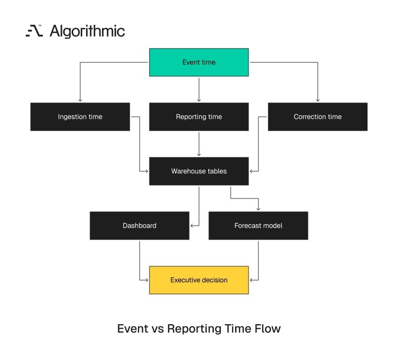
The executive problem is direct. Leaders make decisions at a specific time, using the data available at that time. Most warehouses store corrected history, which differs from the incomplete state leaders saw at the decision point. This split between when an event is valid and when it is recorded is the basis of bitemporal data modeling. Forecasts break when teams train on corrected history and deploy against incomplete reality. A model trained after close sees late invoices, reversed cancellations, and corrected product events. A live forecast issued before close does not have those records.
The difference creates an avoidable accuracy gap. It also creates an accountability problem. Teams argue about tools, models, and dashboards while the source of error sits in the calendar logic.
The four clocks behind most forecast errors
Operational data rarely has one time axis. Most business events carry four clocks. Each clock answers a different business question and supports a different control.
| Clock | Field examples | Business question answered | Common failure mode |
|---|---|---|---|
| Event time | order_created_at, ticket_opened_at, claim_occurred_at | When did the activity happen? | Late-arriving records rewrite historical trends |
| Ingestion time | loaded_at, received_at, Kafka offset timestamp | When did the platform receive the record? | Backfills create artificial spikes |
| Reporting time | posted_at, closed_month, reporting_period | When did the organization report it? | Finance and operations disagree on period totals |
| Correction time | updated_at, reversed_at, adjusted_at | When did the record change after initial capture? | Cohorts move after executive review |
A revenue dashboard grouped by event_time gives one answer. A board metric grouped by reporting_time gives another. A forecast training set built from ingestion_time gives a third. Those answers can pass local validation and still mislead the executive team. SQL tests confirm that rows exist, joins work, and totals reconcile to a selected source. They do not confirm that the metric uses the right clock for the decision.
Finance closes books on posting periods. Sales manages pipeline by signature date. Operations schedules labor by expected service date. Product analytics tracks usage by event time from Segment, Snowplow, Amplitude, or application logs. Support measures ticket volume by opened time and service levels by response time. Customer success measures churn by service end date, cancellation notice date, and renewal date.
A shared warehouse does not reconcile those clocks on its own. The warehouse stores timestamps. The organization must define which timestamp governs each decision. The practical risk appears when two teams use the same label for different clocks. A metric named “revenue” can mean contracted value, invoiced value, recognized revenue, or collected cash. Each version belongs in a different management conversation.
The same pattern applies to customer counts. A customer can sign in March, start service in April, produce first usage in May, and pay in June. A single customer_month field hides the choice that determines the reported result.
Production analytics requires explicit time semantics. The model must state the business role of each date. The test suite must verify that role before the metric reaches an executive table.
 Click to expand
 The failure story of one expansion across three months
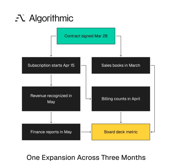
The SaaS company’s forecast miss came from a normal enterprise expansion. The account signed a $2.4 million annual expansion on March 28. The subscription started on April 15 after procurement and provisioning.
Finance recognized the first revenue in May after the contract moved through the close process. Sales operations treated the expansion as March bookings. Billing treated it as April contracted run rate.
Finance treated it as May revenue. Each treatment matched the team’s operating responsibility. The failure came from a metric label that made the treatments look interchangeable.
 Click to expand
 The board deck used a metric labeled “Expansion ARR.” In one table, it pulled from Salesforce close date. In a cash planning sheet, it pulled from billing start date. In a forecast training table, it used the first month with recognized revenue.
No one had written a defective query. Each team selected the date that matched its operating process. The error came from reusing the same metric name across three different time bases. The forecast model learned from historical rows after all corrections had landed. During the live quarter, it scored accounts before billing and revenue recognition had caught up. The model saw less expansion signal than the backtest had promised.
The company’s data team first investigated Looker Explores, dbt dependency chains, and Snowflake performance. They found small issues and fixed them. The forecast variance remained. The decisive finding came from a simple table. For each expansion, the team placed signed date, billing start date, revenue recognition date, and forecast cutoff date in adjacent columns. The variance concentrated in deals where those dates crossed month or quarter boundaries.
That artifact changed the discussion. The issue became a specific operating rule. Expansion reporting needed separate metrics for signed bookings, billed ARR, and recognized revenue. The team then rebuilt the executive table with three columns instead of one. March showed the signed expansion. April showed billed run rate. May showed recognized revenue.
The revised table did not change the business result. It changed the operating interpretation. Leaders could see the bridge from contract execution to billing to accounting treatment. The same fix changed the training data. The model no longer learned from recognized revenue when the forecast required signed expansion signal. The team trained the forecast using the same cutoff and date basis used in production.
That alignment reduced the gap between backtest performance and live performance. It also reduced quarter-end reconciliation time. Finance, RevOps, and analytics engineering stopped debating which dashboard was correct.
Tool migrations leave temporal ambiguity intact
A BI migration can improve access control, governed metrics, and dashboard development. A warehouse migration can increase query concurrency and lower processing time for high-volume tables. A move from batch ETL to event streams can reduce latency. Those changes do not define whether a refund belongs to the order month, refund month, or accounting close month. That definition needs a business rule, a tested model, and a named owner. The rule must exist before the platform can apply it.
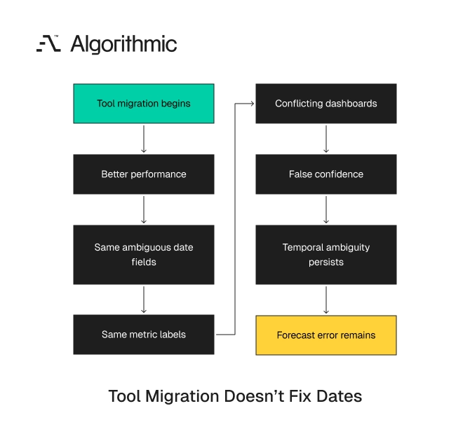
A platform migration often exposes the problem because faster systems update inconsistent metrics sooner. The organization gets fresher disagreement. The executive discussion moves from stale dashboards to conflicting dashboards. A team can move from Tableau to Looker and keep the same ambiguous field names. It can move from Redshift to Snowflake and keep the same incremental load logic. It can add dbt tests and still test only nulls, uniqueness, and accepted values.
The problem survives because it is semantic. The warehouse can process a timestamp. It cannot infer the business event that timestamp represents. A migration can also create false confidence. Teams see cleaner lineage graphs, faster builds, and stricter deployment checks. Those gains matter, and they remain incomplete without time contracts.
A metric that groups refunds by created_at will keep doing so after the migration. A model that loads changes by updated_at will still mix correction time with event time. A dashboard that labels both as “month” will keep misleading readers.
 Click to expand
 The dashboard layer cannot infer business time
BI tools operate on modeled fields. If bookings_date means signed date in one model and finance-posted date in another, the visualization layer renders both with confidence. The chart has no way to know that the same label hides two rules.
Executive dashboards can look precise while carrying structural error. A trend line with two decimal places will not reveal that February includes nine days of late January activity. A variance table with green and red indicators will not show that one measure uses closed_month and another uses contract_start_date. The issue grows when operating teams own separate processes. Sales operations tracks opportunity stage changes by CRM update time. Finance tracks revenue by posting period. Customer success tracks churn by service end date.
Product analytics tracks usage by event time. Support tracks ticket service levels by opened, assigned, first response, and resolution timestamps. RevOps tracks pipeline velocity by stage entry date and close date. Each team follows a rational operating model. The combined reporting layer becomes unstable without explicit time contracts. The instability appears during planning, close, and board preparation.
The defect often enters through naming. A field called date invites misuse. A field called revenue_recognition_month forces the accounting rule into the open. A field called month should fail review in a production metric model. It hides the clock. A production model should name the business role of the date.
Examples include contract_signature_date, billing_start_date, service_period_start_date, posted_accounting_month, and forecast_decision_cutoff_at. These names make the rule visible in code review. They also reduce the chance that a BI author selects the wrong field under deadline pressure. Dashboard labels should carry the same discipline. “Expansion ARR by month” is incomplete. “Signed expansion ARR by contract signature month” gives the reader the clock and the measure.
Finance exports need the same treatment. A spreadsheet tab named “April revenue” should state whether April means service month, invoice month, cash receipt month, or close period. The extra words prevent hours of reconciliation.
Warehouse architecture can preserve the wrong rule
Modern warehouse architecture makes temporal inconsistency easy to replicate. Snowflake, BigQuery, Databricks, and Redshift can process large backfills quickly. dbt can rebuild hundreds of derived tables in one run. That speed helps after teams define time semantics. It increases damage when teams leave time undefined. A data team can rebuild 400 models overnight and preserve the same ambiguity across every derived metric.
The compute bill changes. The decision error remains. Faster execution spreads the wrong definition across more dashboards, exports, and model features. The 2026 State of Analytics Engineering Report from dbt Labs reported that trust in data and data teams rose from 66% to 83% as an organizational priority. Speed rose from 50% to 71%. The same report found that 57% of respondents saw increased warehouse and compute spend.
More compute does not create temporal correctness. It processes the selected semantics at greater scale. If the semantics are wrong, the platform returns the wrong answer faster. This is why forecast error often survives a tool migration. The system becomes cleaner, faster, and more governed at the platform level. The business still lacks a rule for how time enters the metric.
Warehouse design can make the rule easier to apply. Event tables can preserve source timestamps, ingestion timestamps, and correction timestamps. Dimensional models can expose the right date basis for each metric. The architecture still needs a business decision. Engineers can model order_created_at, order_paid_at, order_refunded_at, and revenue_posted_month. Finance must define which field governs the board metric.
A strong platform stores all clocks and prevents destructive overwrites. A weak platform collapses them into one date. Once that collapse occurs, every downstream model inherits the ambiguity.
Temporal defects produce credible reports
Data quality failures such as null customer IDs and duplicate primary keys are visible. Temporal defects are harder to detect because the reports look credible. The output usually has defensible SQL, a familiar chart, and a stable owner. A weekly demand forecast can degrade because 18% of purchase orders arrive after the weekly planning cut. A cohort retention dashboard can overstate Month 2 retention because reactivations attach to the original signup month. A claims forecast can understate incurred losses because the model trains on paid date instead of occurrence date.
Each output has defensible SQL. Each output can pass row-count checks. Each output can match one team’s operating definition. The defect appears during reconciliation. Finance asks why April actuals changed in June. Operations asks why last week’s forecast became accurate after restatement and inaccurate when used for staffing.
The executive team asks why two reports built from the same warehouse show different quarter-to-date revenue. The data team reviews joins, filters, and dimensions. The source of the variance usually sits in the date basis. This makes temporal defects expensive. They consume senior attention during the shortest decision windows. They also damage trust because the numbers disagree after formal review.
A defect in a primary key fails loudly. A defect in a clock fails quietly. It produces a number that looks reasonable until another process presents a different number.
Late-arriving data rewrites the baseline
Late-arriving data changes the past. This behavior is normal in payments, logistics, healthcare, insurance, and B2B revenue operations. The data is late because the business process is late. Retailers receive marketplace settlement data several days after the transaction. Manufacturers receive plant telemetry after network downtime. Healthcare payers receive claims weeks after service.
A SaaS company can book a contract in Salesforce before billing starts in Stripe, Chargebee, or NetSuite. The signed date supports bookings. The billing start date supports cash planning. The revenue recognition date supports GAAP reporting. The forecast cutoff date records what management knew when the forecast was issued. Those four dates should never share one generic field.
Forecasting models trained on fully backfilled history learn from a cleaner world than the one available at decision time. That creates lookahead bias. The model looks accurate offline and degrades in production. The training table often contains corrected outcomes that were unavailable when leaders made the original decision. A model trained on those records learns from future knowledge. The offline backtest then overstates live performance.
This problem appears in manual forecasting as well. A spreadsheet built after close includes late invoices and corrected cancellations. A forecast issued before close did not have that information. The comparison is unfair unless the analysis reconstructs the decision state. Teams need to evaluate forecasts using the data available at the original cutoff. Corrected history should remain available, with a separate view for as-of analysis.
An as-of view preserves what the organization knew at a point in time. It records the state of each record at the forecast cutoff. It lets teams compare the forecast against the data that existed when the decision was made. This method changes how teams review accuracy. The question becomes whether the forecast used the right inputs at the right cutoff. The review no longer rewards models for seeing records that arrived later.
Backfills create artificial trend breaks
Backfills are necessary. They correct source defects, add missing records, and align historical definitions. They also create false movement when ingestion time and event time are mixed.
A backfill of historical product events can appear as a sudden usage spike if a downstream model groups by load date. A correction to 11 months of invoice records can make current-quarter revenue appear to change overnight. A claims load from a clearinghouse can inflate current-week loss volume when the service dates belong to prior months.
This defect appears often during analytics system development. The data platform records when data arrived. The business report needs the activity date and the correction date.
Those dates serve different controls. The activity date supports trend analysis. The correction date supports auditability.
The reporting date supports close management. A mature warehouse stores all three and names each one. A weak warehouse overwrites one with another and loses the audit trail.
Once the audit trail is gone, reconciliation becomes manual. Analysts search through source exports, warehouse snapshots, and Slack messages. Executives wait for the answer while the decision window closes.
The fix is straightforward at the model level. Store event_occurred_at, source_updated_at, ingested_at, effective_from_at, and corrected_at where the process needs them. Downstream marts should select the right timestamp by metric, not by convenience.
Backfills also need a declared operating treatment. A historical correction can update past trend lines, current reports, or a separate restatement table. The choice should be explicit before the load runs.
Teams should tag backfilled records with batch identifiers. They should record load reason, source ticket, affected period, and approval owner. Those fields shorten post-load review when a metric moves.
Attribution windows change period totals
Attribution windows define how long an event remains eligible to influence an outcome. They are temporal business rules. They belong in metric definitions, model code, and tests.
A marketing team can attribute conversions to campaigns within seven days. Sales can attribute expansion to the account owner at contract signature. Finance recognizes revenue across the contract term.
Product can attribute activation to the first successful workflow within 14 days. Support can attribute retention to a save motion completed within 30 days of cancellation risk. Customer success can attribute renewal health to usage changes during the 90 days before contract end.
When those windows are undocumented, dashboards disagree by design. Marketing claims pipeline sourced in March. Sales claims the same expansion in April.
Finance recognizes the revenue across the contract term. Each view serves a purpose. The organization needs distinct metric names, distinct date bases, and a documented reconciliation path.
Planning cycles expose the gap. A chief revenue officer sees sourced pipeline above target. The CFO sees recognized revenue below plan.
Both teams can be right within their own windows. The executive risk comes from comparing them as if they shared one clock. The metric layer should block that comparison unless a reconciliation table exists.
Attribution windows also affect machine learning features. A 30-day usage feature and a 90-day health feature encode different time assumptions. A model review should state those windows beside accuracy metrics.
For executive reporting, attribution windows need owner approval. Marketing can own campaign attribution rules. Finance should approve revenue timing. Customer success should approve renewal health windows.
The framework for temporal contracts in production metrics
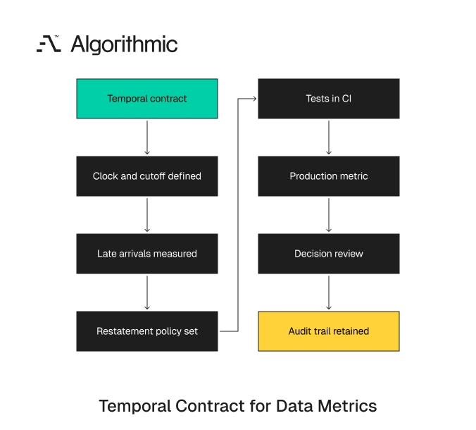
A temporal contract is a written and tested definition of how time behaves in a production metric or model feature. It sits beside schema contracts, freshness service levels, and metric definitions. It states which clock governs the metric, which records arrive late, and which periods can be restated.
Temporal contracts should live in the repository with the model code. They should run in CI through dbt tests, SQL checks, or warehouse-native data tests. They should be visible to finance, operations, RevOps, and analytics engineering. Treating time as a governed part of analytics and business intelligence keeps these rules in the metric layer instead of scattered across individual reports.
The contract applies to dashboards and model features. A board metric and an ML feature can share a source table and still need different time rules. A board metric freezes at close; a staffing forecast freezes before the shift schedule is published.
A contract should fit on one page. If it needs 12 pages, the metric is not ready for production use. The goal is a readable operating artifact, not documentation volume.
The contract should use plain field names and direct ownership. It should state the clock, cutoff, lateness window, and restatement rule. It should also state what happens when the rule is violated.
A useful contract answers the questions asked during an incident. Which period changed? Was the change allowed? Who approved the restatement? Which dashboard and forecast consumed the changed value?
 Click to expand
 A practical temporal contract
For each production metric or model feature, define these fields:
| Contract field | Required decision |
|---|---|
| Business event timestamp | Which timestamp represents the activity being measured |
| Source system timestamp | Which timestamp came from Salesforce, NetSuite, Stripe, SAP, Segment, or the operational database |
| Ingestion timestamp | When the data platform received the record |
| Effective timestamp | When the record starts affecting reporting |
| Correction timestamp | When a value changed after first arrival |
| Allowed lateness window | The delay threshold before a record is treated as late |
| Restatement policy | Which periods can be recalculated after close |
| Attribution window | The interval that links cause and outcome |
| Freshness SLO | p50, p95, and p99 delay from source event to production table |
| Decision cutoff | The moment when the report or forecast freezes input data |
| Owner | The team accountable for the rule |
| Violation handling | Alert, quarantine, restate, or exclude the record |
| Audit record | Where approvals, batch IDs, and restatement notes are stored |
This artifact prevents a common failure. Teams define metric names and formulas while leaving time undefined. A formula without a time basis is incomplete. The contract should name the owner for each rule. Finance owns revenue recognition periods and restatement thresholds. Sales operations owns opportunity stage timing.
Data engineering owns ingestion timestamps and materialization latency. Analytics engineering owns the model implementation and tests. Operations owns staffing cutoffs and service calendars. Ownership matters during incidents. If April revenue changes after close, the team needs to know whether the change violated policy. The answer should come from the contract, not a Slack thread.
Contracts should also define allowed exceptions. For example, finance can permit a closed-period adjustment after a legal correction. Operations can permit late orders to enter a staffing model only before schedule publication. Exception rules need audit fields. A record should show who approved the exception, when approval occurred, and which period changed. That evidence protects the metric during board and audit review.
A contract example for expansion ARR
A production metric called expansion_arr_signed should use contract signature date as the business event timestamp. It should exclude expansions without an approved contract. It should permit restatement only when a contract is reversed or corrected by legal operations. A production metric called expansion_arr_billed should use billing start date. It should reconcile to Stripe, Chargebee, NetSuite, or the billing system of record. It should carry a freshness SLO tied to billing system posting time.
A production metric called expansion_revenue_recognized should use accounting period. It should reconcile to the finance close process. It should freeze after close except for approved restatement entries. Those three metrics can reference the same customer and contract. They should not share one dashboard label. The label should state the date basis in plain language.
A board table can show all three if leaders need the bridge. The bridge should reconcile signed expansion to billed expansion to recognized revenue. That table turns disagreement into an operating view. The same pattern applies to churn. churn_notice_date, service_end_date, billing_end_date, and revenue_churn_month answer different questions. A customer can give notice in March, lose service in April, stop billing in May, and hit revenue reporting in June.
Churn reporting needs separate measures for each management question. Customer success needs notice timing to manage intervention. Finance needs revenue churn month to manage plan variance. Billing needs billing end date to manage collections and invoice accuracy. Product needs service end date to study usage decay before departure. A single churn month cannot serve all four questions.
The contract also improves sales compensation review. If a rep receives credit at signature, the compensation table should use signature date. If finance reports revenue over the term, that table should use accounting periods. Mixing those clocks creates compensation disputes. Separating them gives sales, finance, and the board one reconciliation path. The bridge table becomes the shared evidence base.
Freshness SLOs must be measured at the feature and metric level
“Daily refresh” is not an engineering requirement. It does not state when the source event occurred. It does not state when the record arrived, transformed, or reached the dashboard.
A useful freshness SLO reads this way: 95% of paid invoice events must appear in the finance_revenue_daily mart within four hours of NetSuite posting. The same SLO can state that 99% must appear within 12 hours. It should specify whether the clock starts at event creation, source update, ingestion, or accounting post. Tools such as dbt source freshness checks encode these thresholds as warn and error windows per source.
For ML systems in production, this measurement must reach the feature layer. A churn model using 30-day usage counts should report p50, p95, and p99 latency from product event ingestion to materialized feature. A recommendation system using hourly aggregates should state which windowed aggregates are supported and how late events are treated. Vendors and internal platform teams should be judged on those numbers. A partner that cannot provide latency and correctness metrics for feature delivery has not proven production maturity. A team that cannot measure feature staleness cannot manage forecast reliability.
The metric also needs a declared failure mode. If p99 latency exceeds 12 hours, the pipeline should alert the owner. If a feature misses the decision cutoff, the forecast should record that condition in the output table. This record matters during forecast review. A forecast with stale usage features should not be compared to a forecast with current usage features as if they had equal inputs. The review should show which cutoff and feature state produced each forecast.
A production forecast table should include forecast_generated_at, decision_cutoff_at, feature_as_of_at, and training_data_as_of_at. Those columns give executives and engineers the evidence needed to explain a variance. They also prevent the team from rerunning history with data that was unavailable at decision time.
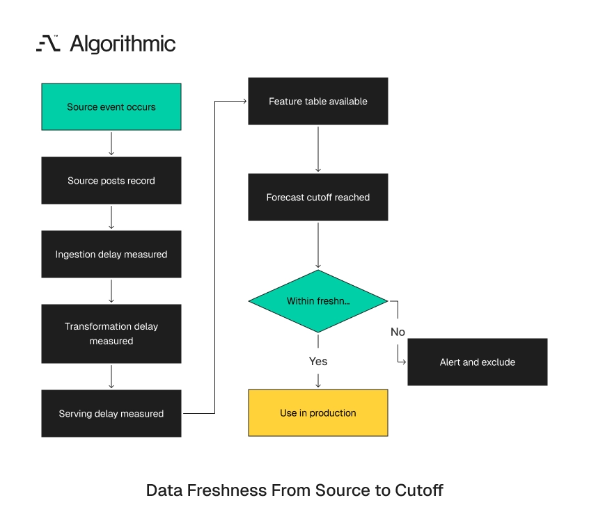 Click to expand
 Freshness should be measured per source and per derived table. Product events, billing events, CRM updates, and support tickets arrive through different paths. A single warehouse freshness number hides the system that failed. Feature stores need the same discipline. A feature named usage_30d should state whether the 30-day window ends at event time, ingestion time, or forecast cutoff. The materialized table should carry the timestamp used for that window.
Without that timestamp, evaluation becomes unstable. A model can look stronger after a rerun because late product events enter the historical feature window. The forecast then receives credit for information it did not have in production. A strong SLO ties the feature to the decision. For example, a staffing forecast published Monday at 10:00 a.m. should freeze all order inputs at Monday 8:00 a.m. Late orders should be logged and excluded from that forecast run.
The exclusion does not hide the late orders. It records them in a separate lateness table. That table helps operations adjust planning rules and helps engineering improve source delivery.
Causal reporting requires stronger time records
Forecasting and operational reporting become more complex when leaders want causal answers. Did a price change reduce churn? Did a new onboarding flow increase activation? Did the sales incentive plan pull deals forward from next quarter? Those questions need more than outcome timestamps. They need assignment records, exposure timestamps, eligibility rules, and outcome observation windows. They also need a record of what the organization knew before the action.
Causal analysis needs action assignments, pre-treatment covariates, and outcome timelines. The platform must record who received the intervention. It must record when the assignment was made and what was known before assignment. It must also record when each outcome became observable. Without those records, teams confuse timing effects with treatment effects. A campaign can appear effective because high-intent accounts were assigned earlier.
A workflow change can appear neutral because adoption was measured before the lag window closed. A retention program can appear successful because canceled accounts had not reached their billing end date. A pricing change can appear to increase ARR because renewals were pulled forward into the measurement window. This matters for forecasting. A model trained on outcomes without assignment timelines learns from post-treatment data. That contaminates evaluation and produces forecasts that fail when the intervention changes.
Consider a retention model trained after a save campaign. If the training data includes post-campaign product usage, the model learns behavior caused by the intervention. The next campaign changes assignment rules, and the model loses calibration.
The fix requires time-aware instrumentation at the moment of action. The system should record eligibility, assignment, exposure, and outcome windows. Those records should feed causal reporting and forecast training tables. A practical action table includes entity_id, eligible_at, assigned_at, exposed_at, action_type, assigned_by, assignment_rule_version, and outcome_observation_ends_at. That table gives analytics teams the ability to separate who was eligible, who was selected, who was exposed, and when results were observable. It also gives executives a record they can audit.
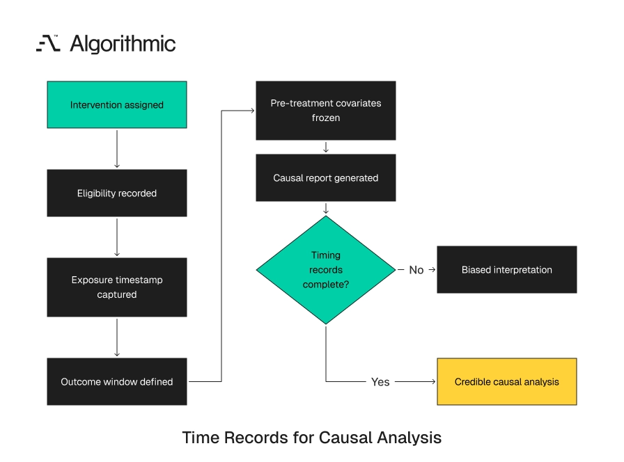 Click to expand
 Causal reporting also needs stable exclusion rules. If an account was ineligible at assignment time, later eligibility should not rewrite the experiment population. The original assignment state must remain available. This requirement applies outside formal experiments. A sales manager can assign accounts to a renewal playbook. A support leader can assign tickets to a premium queue.
Both actions create exposure records. Both can change future behavior. Forecast models should know whether an outcome occurred before or after the operational action. A disciplined action table prevents post hoc explanations from replacing evidence. It also lets leaders compare actions across cohorts. The comparison works only when the timing of assignment, exposure, and outcome is recorded.
A 30-day temporal alignment audit
A temporal alignment audit should take 30 days for a mid-sized data platform with 50 to 150 production models. The goal is to identify metrics and features where date semantics create decision risk. The output should be contracts, tests, and a ranked remediation backlog. The work should involve analytics engineering, finance, operations, RevOps, and source-system owners. Temporal definitions sit across business process and data code. A data-only review misses policies embedded in close calendars, sales compensation plans, and staffing rules.
This audit should not start with the entire warehouse. It should start with decision-facing assets. Board metrics, cash forecasts, staffing plans, and customer health measures carry the highest executive risk. The audit should use a small senior team. A typical team includes one analytics engineer, one data engineer, one finance owner, one RevOps owner, and one operations owner. A technical program lead should maintain the register and drive decisions.
The group should meet twice weekly for 45 minutes. Most work happens in the repository, warehouse, BI tool, and source systems. The meetings resolve ownership and approve rules.
Week 1 inventory decision-facing assets
List the dashboards, forecasts, and operational reports used in executive, finance, and staffing decisions. Rank them by decision value and usage frequency. A weekly staffing forecast carries a different risk profile than an exploratory adoption chart. For each asset, record the primary date field, filter date, refresh cadence, owner, and downstream surfaces. Most mid-sized organizations find 20 to 40 high-value assets that drive most recurring decisions. The inventory should include board deck tables, finance exports, spreadsheet models, and operational queues.
Record where each metric appears. A revenue measure used in Looker, Google Sheets, and a board presentation should be treated as one decision asset with multiple surfaces. This prevents teams from fixing a dashboard while leaving the export unchanged. The artifact for Week 1 is a decision asset register. It should list the metric, owner, source model, date field, decision owner, and decision cadence. This register becomes the audit scope.
The register should also identify the decision made from each asset. “Board review” is too broad. “Approve hiring plan,” “revise cash forecast,” or “set weekly staffing levels” gives the metric a business consequence. That consequence drives prioritization. A metric used to approve a $4 million hiring plan deserves review before a dashboard used for exploratory segmentation. Decision value should govern the order of work.
Week 2 trace timestamp lineage
Trace each high-value metric from dashboard to warehouse model to source system. Identify every timestamp used in joins, filters, aggregations, snapshots, and incremental loads. Include BI calculated fields and spreadsheet transformations. This step often reveals silent substitutions. A model filters invoices by created_at, joins payments by updated_at, and reports by posted_period. Each timestamp has a valid role.
The model needs to state which role it serves. If the metric is recognized revenue, posted_period should govern reporting. If the metric is bookings, signature date or opportunity close date should govern reporting. Lineage should include incremental logic. A table that loads records where updated_at > max(updated_at) follows correction time. A dashboard grouped by created_at then mixes correction logic with event reporting.
The artifact for Week 2 is a timestamp lineage map. It should show every clock used by the metric and the point where one clock changes to another. That map usually exposes the highest-risk defects. The map should include source-system behavior. Salesforce opportunity close date can be edited after the deal closes. NetSuite posting periods can close and reopen under controlled conditions.
Stripe event creation time, webhook delivery time, and warehouse load time can differ by minutes or hours. Product event timestamps can reflect client device time, server receipt time, or collector time. Those differences matter during cutoffs and backfills.
Week 3 quantify lateness and restatement
Measure arrival delay for each source. Calculate p50, p95, and p99 lag from event time to ingestion time. Then calculate lag from ingestion time to the materialized reporting table. Measure restatement volume as well. For closed periods, count how many records changed after one day, seven days, 30 days, and quarter close. A finance metric that changes by 0.2% after close carries a different risk profile from one that changes by 6%.
Break the numbers down by source system and business process. NetSuite postings, Stripe events, Salesforce opportunities, Zendesk tickets, and product events follow different lateness patterns. A single platform-level freshness number hides the operational cause. The output should include a lateness distribution for each decision asset. Averages are insufficient. A p95 delay of four hours and a p99 delay of three days require different staffing and close controls.
The artifact for Week 3 is a lateness and restatement report. It should show which metrics change after the decision date and by how much. It should also identify sources that miss the stated decision cutoff. This work often changes executive expectations. A metric that is 99% complete after four hours can support same-day decisions. A metric that receives 8% of records after three days should not drive a daily operating review.
The report should separate normal lateness from defect-driven lateness. Normal lateness follows the business process, such as insurance claims received after service. Defect-driven lateness comes from pipeline failures, source outages, or missed schedules.
Week 4 set contracts and tests
Write temporal contracts for the top 10 decision assets. Add tests that fail when records exceed expected lateness, when closed periods change beyond threshold, or when required timestamps are null. The first contracts should cover board metrics, cash planning, staffing forecasts, and customer health measures. Add dashboard labels that state the time basis: event date, posted date, report date, or decision cutoff. This small change reduces reconciliation time because teams stop comparing metrics built on different clocks. It also gives executives a clear reason for differences between reports.
Add dbt tests or warehouse checks for contract violations. A test can fail when posted_period is null for recognized revenue. Another can fail when a closed period changes by more than the approved basis-point threshold. Model features need the same checks. A feature table should store feature_as_of_timestamp, source window, and materialization time. Forecast evaluation should use the same decision cutoff that production used.
The artifact for Week 4 is a remediation backlog. Rank each issue by decision risk, forecast effect, and engineering effort. Fix naming, contracts, and tests before large model rewrites. The backlog should separate four classes of work. Naming fixes clarify fields and labels. Contract fixes define the business rule. Test fixes detect violations. Model fixes change the transformation logic.
This separation prevents overbuilding. Many defects need a contract and label change before code changes. Some defects need new snapshot tables, effective dating, or feature-store changes. The final audit readout should fit in 10 slides. It should show the top assets, top clock conflicts, lateness distributions, restatement exposure, and approved remediation plan. The executive team needs decisions, owners, and dates.
Use this decision matrix before changing tools
Tooling changes have a place. They should follow temporal diagnosis. The matrix below separates semantic defects from platform constraints.
| Symptom | Temporal cause | Engineering response | Tool change required |
|---|---|---|---|
| Forecast accuracy is strong offline and weak in production | Training data includes late corrections unavailable at decision time | Rebuild training sets using decision cutoffs | No |
| Month-end reports change after close | Corrections lack restatement policy | Add effective dates and closed-period controls | No |
| Sales and finance dashboards disagree | Signed date and posted date are mixed | Define separate metrics for bookings and recognized revenue | No |
| Usage spikes after data recovery | Backfill loads by ingestion date | Separate event time from load time in marts | No |
| Dashboards are slow and definitions are consistent | Query patterns exceed current warehouse design | Partition, cluster, or remodel high-volume tables | Possible |
| Feature freshness misses operational decision windows | Pipeline latency exceeds SLO | Measure p95 and p99 delay across ingestion, transformation, and serving | Possible |
| Cohort retention changes after review | Reactivations attach to original signup period | Add effective-dated cohort membership rules | No |
| Staffing forecasts miss weekly demand | Orders arrive after the planning cutoff | Freeze forecast inputs and track late arrivals | No |
| Board metrics differ from finance exports | Dashboard uses event date and finance export uses close period | Publish a reconciliation bridge | No |
| ML model retraining changes historical accuracy | Training set uses corrected outcomes | Store as-of snapshots for training and evaluation | No |
| Customer health scores change after QBR prep | Late usage events enter the measurement window | Freeze QBR inputs and log late-arriving events | No |
| Cash forecast misses collection timing | Invoice date and expected cash date are treated as one field | Model invoice, due, payment, and receipt dates separately | No |
This matrix prevents teams from treating every reporting failure as a platform selection problem. It also clarifies when architecture work is justified. Slow queries with consistent definitions call for warehouse design work; inconsistent clocks call for semantic repair. The distinction saves time and money. A $300,000 BI migration leaves a signed-date and posted-date conflict intact. A two-week contract and test effort often resolves the disagreement.
The production answer is practical. Name the clock. Measure lateness. Freeze decision inputs. Record corrections. Test restatement rules. These steps belong in the same engineering system as schema tests and deployment checks. They should run before executive metrics reach production. They should also run before a forecast model is evaluated.
Tool decisions should come after this work. If definitions are consistent and performance remains poor, architecture changes have a clear target. If definitions conflict, a new tool will reproduce the conflict. A good tool evaluation uses temporal requirements as acceptance criteria. The platform must preserve multiple timestamps, support as-of snapshots, expose feature freshness, and test closed-period restatements. Those requirements matter more than dashboard aesthetics.
What leaders should change now
Analytics engineering, finance, and operations leaders should treat time as a modeled domain concept. Date fields should carry business meaning, operating rules, and measured latency. A timestamp without a named business role is a source of reporting risk. Start with the 10 metrics that appear in board decks, cash planning, staffing plans, and customer health reviews. For each one, identify the event date, reporting date, correction policy, attribution window, freshness SLO, and decision cutoff. Then add tests that fail when the data violates those rules.
Assign owners to the time rules. Finance should own close periods and restatement thresholds. Operations should own staffing cutoffs. Analytics engineering should own model implementation and test coverage. Do this before replacing the BI tool, changing warehouse vendors, or adopting a new forecasting model. Temporal alignment explains more variance than tooling choice in the reports that leaders use to run the business. Organizations that fix it gain cleaner forecasts, shorter reconciliations, and fewer executive debates about which number is correct.
The directive is clear for the next operating review. Pick one board metric, one finance forecast, and one operational forecast. Publish the clock, cutoff, lateness profile, restatement policy, and owner for each within 30 days. Then put those rules in production. Add the contract to the repository. Add tests to the deployment path. Add labels to the dashboard and bridge tables to the board package.
The work is small compared with the cost of repeated forecast misses. It gives leaders the evidence needed to trust a number at the moment they use it. It also gives engineering teams a clear boundary between semantic repair and platform investment.
If your board numbers change depending on which team you ask, the fix lives in the metric layer. Algorithmic builds analytics and business intelligence systems where date conventions, freshness SLOs, and temporal contracts are versioned and tested next to the model code. Ask us to audit your forecast pipeline.